Simulating Retail Sales

This tutorial walks you through creating a realistic, multi-dimensional retail sales dataset representing a full year of daily transactions.

Whether you need data to train forecasting models, load-test a database, or build dashboard mockups, this guide shows you how to design complex, multi-layered behaviors that mimic real-world consumer patterns.

---

🎯 The Scenario & Requirements

We want to simulate a retail chain with the following dimensions and behavior parameters:

1. Context Axes (Dimensions)

• store_id: A unique store identifier (e.g. STORE_001, STORE_002, STORE_003).
• product_category: Discrete categorical product departments: Electronics, Apparel, and Home.

2. Numeric Sales Revenue Metrics

Our metric column revenue should model these real-world market behaviors:

• Creeping Growth (Base Trend): Sales should experience linear growth over the year, starting around \$1,000 and ending around \$1,500 daily.
• Weekly Seasonality (Sinusoidal Cycle): Retail traffic peaks heavily on weekends. We need a periodic cycle that peaks every $7$ days with an amplitude of \$200.
• Holiday Sales Surges (Holiday Adjustments): Major US public holidays (like Black Friday, Christmas, and Independence Day) should trigger sharp sales spikes up to \$500 that ramp up in the days leading to the holiday and cool down quickly after.
• Inventory Stockouts (Bursty Gaps): Occasional logistics failures or store closures should trigger consecutive days of zero/NaN revenue.

---

🛠️ Option 1: The CLI & JSON Config Solution (Zero-Code)

You can generate this dataset entirely within your terminal using tsdata.

The Shorthand CLI Command:

tsdata generate \
  --start 2023-01-01 --end 2023-12-31 --granularity D \
  --dims "store_id:auto_generate_name:STORE_" \
  --dims "product_category:Electronics,Apparel,Home" \
  --mets "revenue:LinearTrend(offset=1000,slope=50)+SinusoidalTrend(amplitude=200,freq=7)+HolidayTrend(country='US',effect=500,pre_window=3,post_window=1)" \
  --anomalies "revenue:MissingData(mode=burst,burst_probability=0.01,min_length=1,max_length=3)" \
  --seed 42 \
  --output retail_dataset.csv

The Equivalent JSON Configuration (retail_config.json):

Creating a JSON config is recommended for reproducibility.

{
    "start": "2023-01-01",
    "end": "2023-12-31",
    "granularity": "D",
    "seed": 42,
    "dimensions": [
        "store_id:auto_generate_name:STORE_",
        "product_category:random_choice:Electronics,Apparel,Home"
    ],
    "metrics": [
        "revenue:LinearTrend(offset=1000,slope=5,noise_level=5)+SinusoidalTrend(amplitude=10,freq=7,noise_level=5)+HolidayTrend(country=US,effect=50,pre_window=3,post_window=1)"
    ],
    "anomalies": [
        "revenue:MissingData(mode=burst,burst_probability=0.01,min_length=1,max_length=3)"
    ],
    "output": "retail_dataset.csv"
}

To run this file:

tsdata generate --config retail_config.json

---

🐍 Option 2: The Python API Solution

For pipeline integration, you can compose this exact scenario programmatically.

from ts_data_generator import DataGen
from ts_data_generator.schema.models import AggregationType
from ts_data_generator.utils.functions import auto_generate_name, random_choice
from ts_data_generator.utils.trends import LinearTrend, SinusoidalTrend, HolidayTrend
from ts_data_generator.anomalies import MissingData

# 1. Initialize our year-long daily generator
dg = DataGen(seed=42)
dg.start_datetime = "2023-01-01"
dg.end_datetime = "2023-12-31"
dg.to_granularity("D") # Daily granularity

# 2. Add Dimensions to provide contextual axes
dg.add_dimension("store_id", auto_generate_name("STORE_"))
dg.add_dimension("product_category", random_choice(["Electronics", "Apparel", "Home"]))

# 3. Define and Layer our Revenue Trends
growth_trend = LinearTrend(offset=1000.0, slope=5.0, noise_level=5.0) # Steady growth with some noise
weekly_seasonality = SinusoidalTrend(amplitude=10.0, freq=7.0, noise_level=5.0) # Period = 7 days for weekly cycle
holiday_spikes = HolidayTrend(country="US", effect=50.0, pre_window=3, post_window=1)

revenue_trends = {growth_trend, weekly_seasonality, holiday_spikes}

# 4. Define our Inventory Stockout anomaly
stockout_dropout = MissingData(
    mode="burst", 
    burst_probability=0.01, 
    min_length=1, 
    max_length=3
)

# 5. Attach the completed metric
dg.add_metric(
    name="revenue",
    trends=revenue_trends,
    aggregation_type=AggregationType.SUM, # Revenue is summed when resampling!
    anomalies=[stockout_dropout]
)

# 6. Retrieve the generated Pandas DataFrame
df = dg.data

# 7. Print statistics and sample data
print("--- Simulated Retail Dataset Summary ---")
print(df.info())
print("\n--- First 10 Rows ---")
print(df.head(10))

# 8. Render a quick line chart of our revenue trend
dg.plot(include=["revenue"])

Output: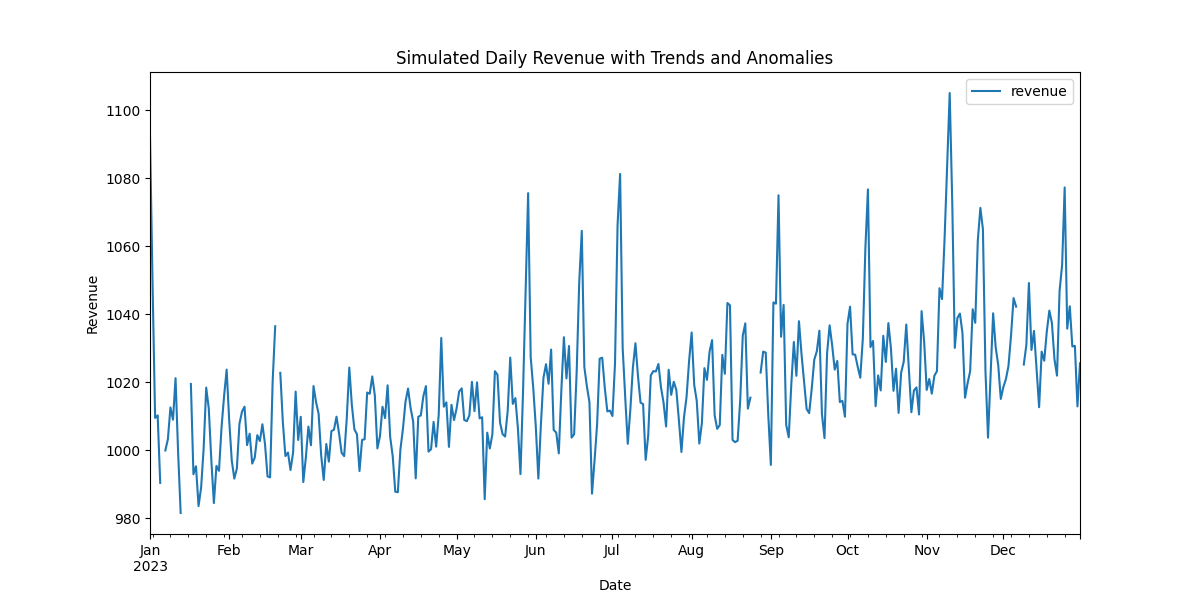

---

🔍 Breaking Down the Business Logic

Let’s dissect exactly why this model maps so closely to real retail stores:

1. SinusoidalTrend(amplitude=10, freq=7): Because our granularity is set to D (daily), specifying a period frequency freq=7 creates a perfect $7$-day wave. This models the weekend shopping boost, where revenue oscillates smoothly between quiet weekdays and busy weekends.
2. HolidayTrend(country='US', effect=500): Automatically looks up federal US holidays (such as Thanksgiving, Christmas, and 4th of July). By setting pre_window=3 and post_window=1, the model simulates the typical pre-holiday buying rush (gradual ramp starting 3 days early) peaking on the holiday itself, before dropping back to baseline the day after.
3. MissingData(mode='burst'): Rather than dropping random individual hours, mode='burst' drops consecutive blocks of days. This simulates physical retail real-world events, such as severe weather, power grid failures, or a product category experiencing a complete supplier stockout for $1$ to $3$ days.