Trend Functions
Trends are the primary mathematical building blocks of metrics in ts-data-generator. Rather than writing complex equations for a metric, you define simple individual Trend components and compose them additively.
The final clean baseline signal is the sum of all its composed trends:
\[\text{Baseline}(t) = \sum_{i} \text{Trend}_i(t)\]📈 Supported Trend Types
Every trend class inherits from Trends and is located in ts_data_generator.utils.trends. Below is the complete catalog of all 7 available trends with their options, Python API usage, and CLI shorthand strings.
1. SinusoidalTrend
Generates periodic sinusoidal waves to model cycles (e.g. daily temperature fluctuations, weekly retail cycles).
amplitude(float): Peak deviation from baseline (default1.0).freq(float): Period of oscillation in days (e.g.,1.0for daily,7.0for weekly).phase(float): Phase offset in hours (default0.0).noise_level(float): Standard deviation of Gaussian noise added to the wave (default0.0).
# API:
from ts_data_generator.utils.trends import SinusoidalTrend
trend = SinusoidalTrend(amplitude=15.0, freq=1.0, phase=6.0, noise_level=0.5)
# CLI Shorthand:
SinusoidalTrend(amplitude=15,freq=1,phase=6,noise_level=0.5)
2. LinearTrend
Generates a steady upward or downward slope with optional white noise.
offset(float): The starting value at $t=0$ (default0.0).slope(float): Angle of the trend in degrees; must be in(-90, 90)(default10.0).noise_level(float): Standard deviation of Gaussian noise (default0.0).
# API:
from ts_data_generator.utils.trends import LinearTrend
trend = LinearTrend(offset=100.0, slope=15.0, noise_level=1.0)
# CLI Shorthand:
LinearTrend(offset=100,slope=15,noise_level=1)
3. WeekendTrend
Creates distinct steps or spikes on weekends (Saturday and Sunday) relative to weekdays.
weekend_effect(float): Magnitude of the weekend shift (default1.0).direction("up"or"down"): Increase or decrease values on weekends (default"up").noise_level(float): Volatility on weekends (default0.0).limit(float): Extreme clamp threshold for the weekend values (default10.0).
# API:
from ts_data_generator.utils.trends import WeekendTrend
trend = WeekendTrend(weekend_effect=50.0, direction="up", noise_level=2.0)
# CLI Shorthand:
WeekendTrend(weekend_effect=50,direction='up',noise_level=2)
4. HolidayTrend
Ramps values up or down around public holidays. It integrates with the holidays Python package for automatic country calendars, or takes explicit dates.
country(str): ISO country code (e.g.,"US","DE","GB") for automatic holiday lookup (default"US").effect(float): Peak adjustment magnitude on the holiday (default50.0).pre_window(int): Number of days before the holiday to start ramping up (default3).post_window(int): Number of days after the holiday to ramp down (default2).direction("up"or"down"): Direction of the holiday adjustment (default"up").dates(list[str]): Custom date strings (YYYY-MM-DD) as fallback/override list.
# API (Automatic US Calendar):
from ts_data_generator.utils.trends import HolidayTrend
trend = HolidayTrend(country="US", effect=100.0, pre_window=3, post_window=1)

# API (Custom Dates):
custom_trend = HolidayTrend(dates=["2024-07-04", "2024-12-25"], effect=200.0)
# CLI Shorthand:
HolidayTrend(country='US',effect=100,pre_window=3,post_window=1)
5. ARNoiseTrend
Generates Autoregressive $AR(p)$ noise: \(X_t = \sum_{i=1}^{p} \phi_i X_{t-i} + \epsilon_t\) This creates realistic “sticky” volatility where today’s fluctuation is correlated with yesterday’s, unlike pure white noise.
coefficients(list[float]): Explicit $AR$ weights $[\phi_1, \phi_2, …]$.decay(float): Alternatively, provide a stable decay factor in $(0, 1)$ to auto-compute stable stationary coefficients.order(int): The order $p$ (lag length) when using thedecayauto-generation (default1).noise_std(float): Standard deviation of the random innovation $\epsilon_t$ (default1.0).
# API (Explicit AR(2) process):
from ts_data_generator.utils.trends import ARNoiseTrend
trend = ARNoiseTrend(coefficients=[0.6, -0.2], noise_std=1.5)

# API (Auto-generated stable AR(3) process):
stable_trend = ARNoiseTrend(decay=0.7, order=3, noise_std=1.0)
# CLI Shorthand:
ARNoiseTrend(coefficients=[0.6,-0.2],noise_std=1.5)
6. MarkovTrend
Simulates discrete regime switches (e.g. system jumping between “Idle”, “Active”, and “Overloaded” states). At each step, it samples the next state and adds minor innovation.
states(list[str]): Categorical names for the discrete states.values(list[float]): Baseline numeric values representing each state.stickiness(float): Probability in $[0, 1]$ of staying in the current state (off-diagonals are distributed equally).transition_matrix(list[list[float]]): An explicit stochastic matrix where rows sum to1.0.noise_std(float): Gaussian noise added to the current state baseline (default0.0).
# API (Stickiness mode):
from ts_data_generator.utils.trends import MarkovTrend
trend = MarkovTrend(
    states=["low", "medium", "high"],
    values=[10.0, 50.0, 150.0],
    stickiness=0.9,
    noise_std=1.0
)

# API (Transition Matrix mode):
matrix_trend = MarkovTrend(
    states=["off", "on"],
    values=[0.0, 100.0],
    transition_matrix=[[0.95, 0.05], [0.10, 0.90]],
    noise_std=0.5
)
# CLI Shorthand:
MarkovTrend(states=['low','medium','high'],values=[10,50,150],stickiness=0.9,noise_std=1.0)
7. StockTrend
A compound financial simulation combining an integrated random walk (Brownian motion) with multi-scale overlapping cycles to simulate realistic equity and asset prices.
amplitude(float): Maximum scale of the price movement (default15.0).direction("up"or"down"): Overall drift direction of the walk (default"up").noise_level(float): Volatility scale of the random walk innovations (default0.0).
# API:
from ts_data_generator.utils.trends import StockTrend
trend = StockTrend(amplitude=100.0, direction="up", noise_level=0.5)
# CLI Shorthand:
StockTrend(amplitude=100.0,direction='up',noise_level=0.5)
🧱 Trend Composition (Layering)
The true power of this architecture comes from composing these trends. Since trends are purely additive, you can layer growth, seasonal cycles, holiday effects, and sticky noise.
Here is a complete, runnable script showing how to build a highly realistic telemetry signal by layering three distinct trends:
from ts_data_generator import DataGen
from ts_data_generator.utils.trends import (
    LinearTrend,
    SinusoidalTrend,
    ARNoiseTrend
)

# 1. Setup Generator
dg = DataGen(seed=42)
dg.start_datetime = "2024-01-01"
dg.end_datetime = "2024-01-14"
dg.to_granularity("h")

# 2. Define our composed layers
base_growth = LinearTrend(offset=50.0, slope=2.0)             # Upward linear crawl
daily_cycle = SinusoidalTrend(amplitude=10.0, freq=1.0)      # Daily sine oscillation (period = 1 day)
network_noise = ARNoiseTrend(decay=0.85, noise_std=2.0)      # Volatility with lag stickiness

# 3. Add to the metric (trends are provided as a set/list)
dg.add_metric(
    name="active_sessions",
    trends={base_growth, daily_cycle, network_noise}
)

# 4. Generate and inspect
df = dg.data
print(df.head(10))

# 5. Visualize composition
dg.plot()
Output: 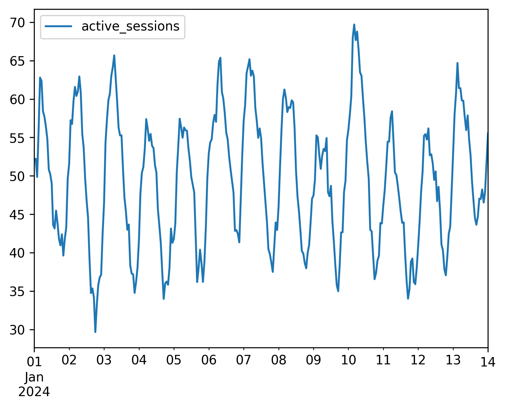
Composing via the CLI
In the command line, use the + operator to stack shorthand trend definitions:
tsdata generate \
  --start 2024-01-01 --end 2024-01-14 --granularity h \
  --mets "active_sessions:LinearTrend(offset=50,slope=2)+SinusoidalTrend(amplitude=10,freq=1)+ARNoiseTrend(decay=0.85,noise_std=2)" \
  --output active_sessions.csv